Everything you need to know about tree data structures

2017-11-05

When you first learn to code, it’s common to learn arrays as the “main data structure.”

Eventually, you will learn about hash tables too. If you are pursuing a Computer Science degree, you have to take a class on data structure. You will also learn about linked lists, queues, and stacks. Those data structures are called “linear” data structures because they all have a logical start and a logical end.

When we start learning about trees and graphs, it can get really confusing. We don’t store data in a linear way. Both data structures store data in a specific way.

This post is to help you better understand the Tree Data Structure and to clarify any confusion you may have about it.

In this article, we will learn:

What is a tree
Examples of trees
Its terminology and how it works
How to implement tree structures in code.

Let’s start this learning journey. :)

Definition

When starting out programming, it is common to understand better the linear data structures than data structures like trees and graphs.

Trees are well-known as a non-linear data structure. They don’t store data in a linear way. They organize data hierarchically.

Let’s dive into real life examples!

What do I mean when I say in a hierarchical way?

Imagine a family tree with relationships from all generation: grandparents, parents, children, siblings, etc. We commonly organize family trees hierarchically.

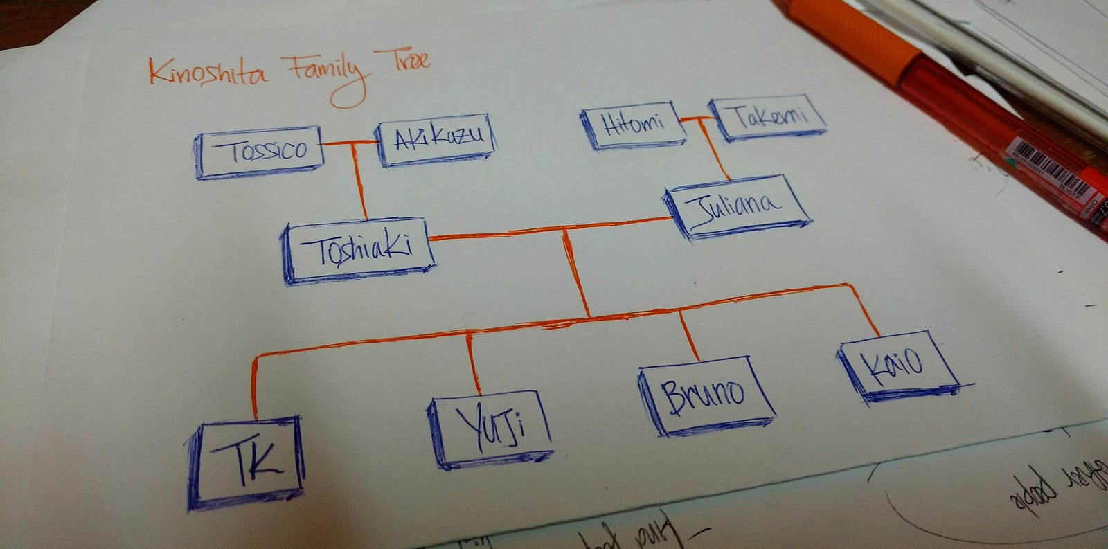
The above drawing is is my family tree. Tossico, Akikazu, Hitomi, and Takemi are my grandparents.

Toshiaki and Julianaare my parents.

TK, Yuji, Bruno, and Kaio are the children of my parents (me and my brothers).

An organization’s structure is another example of a hierarchy.

In HTML, the Document Object Model (DOM) works as a tree.

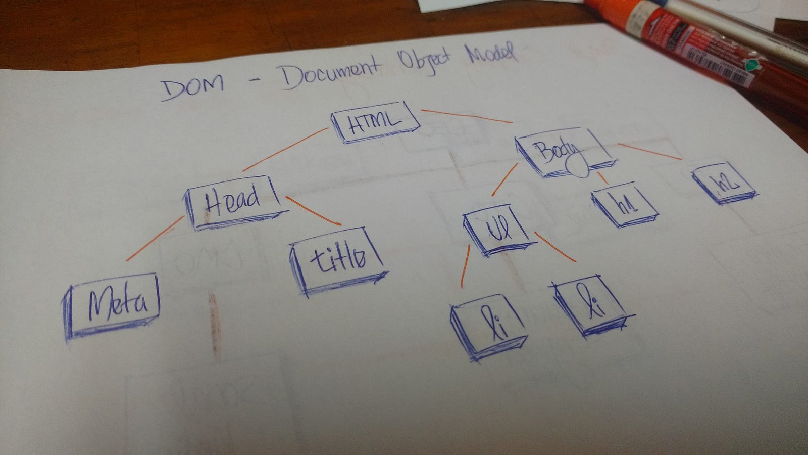
The HTML tag contains other tags. We have a head tag and a body tag. Those tags contains specific elements. The head tag has meta and title tags. The body tag has elements that show in the user interface, for example, h1, a, li, etc.

A technical definition

A tree is a collection of entities called nodes. Nodes are connected by edges. Each node contains a value or data, and it may or may not have a child node .

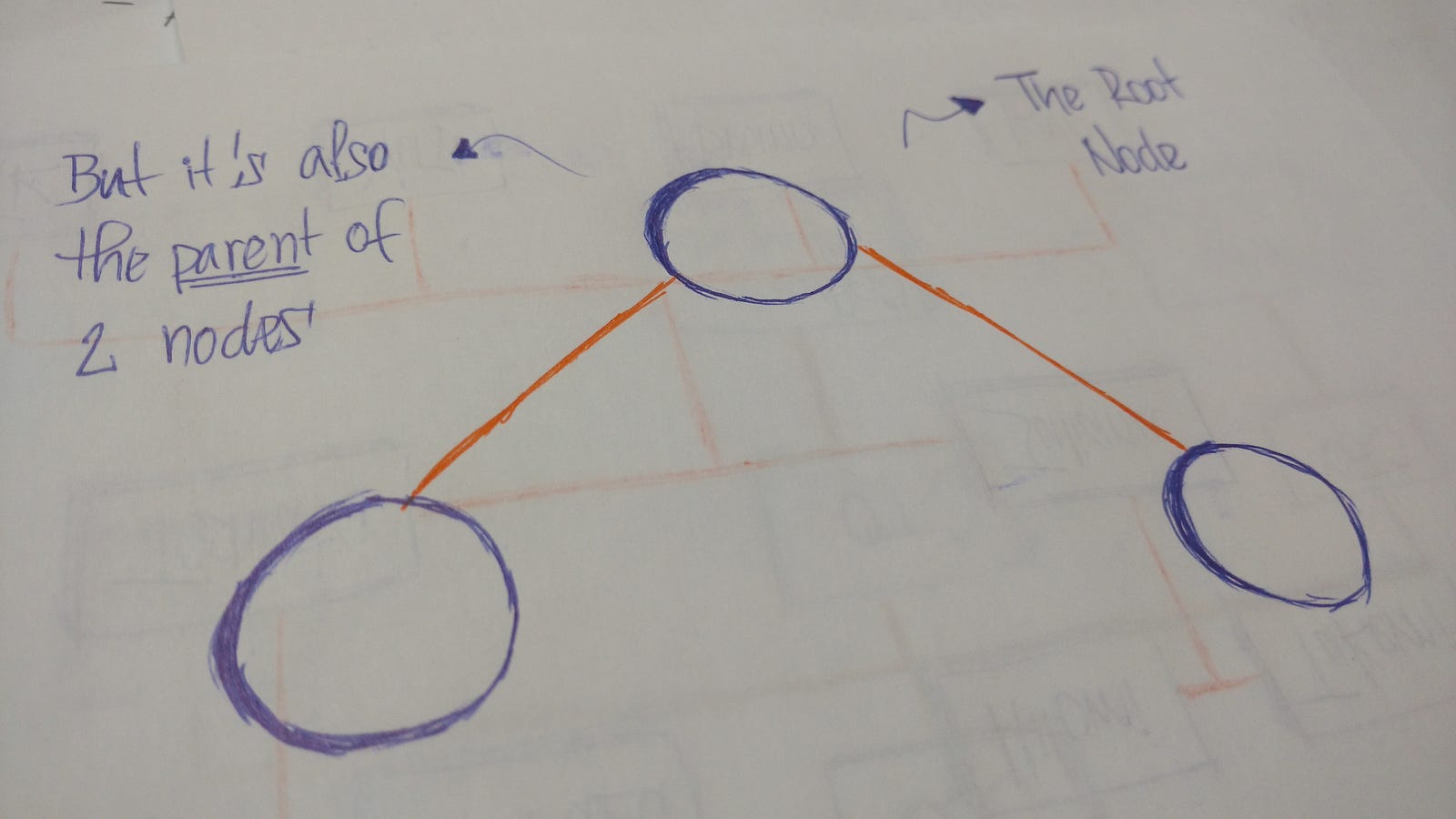
The first node of the tree is called the root. If this root node is connected by another node, the root is then a parent node and the connected node is a child.

AllTree nodes are connected by links called edges. It’s an important part of trees, because it’s manages the relationship between nodes.

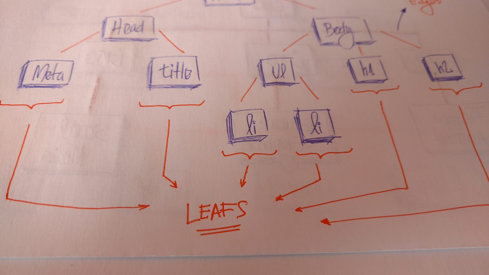
Leaves are the last nodes on a tree. They are nodes without children. Like real trees, we have the root, branches, and finally the leaves.

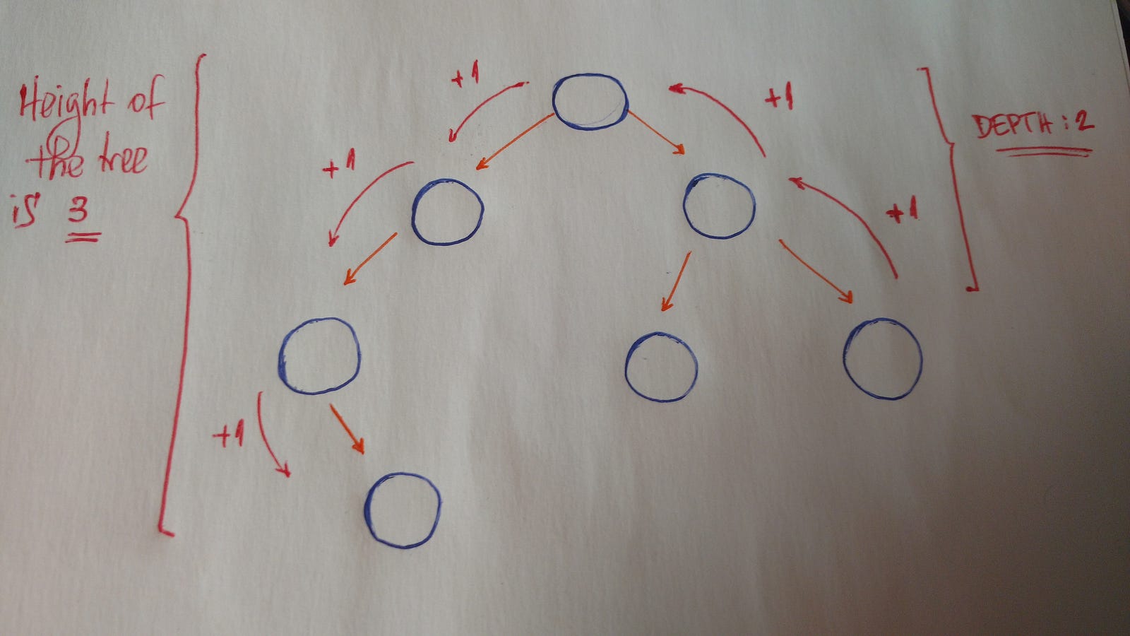
Other important concepts to understand are height and depth.

The height of a tree is the length of the longest path to a leaf.

The depth of a node is the length of the path to its root.

Terminology summary

**Root **is the topmost node of the tree
**Edge **is the link between two nodes
**Child **is a node that has a parent node
**Parent **is a node that has an edge to a child node
**Leaf **is a node that does not have a child node in the tree
**Height **is the length of the longest path to a leaf
**Depth **is the length of the path to its root

Binary trees

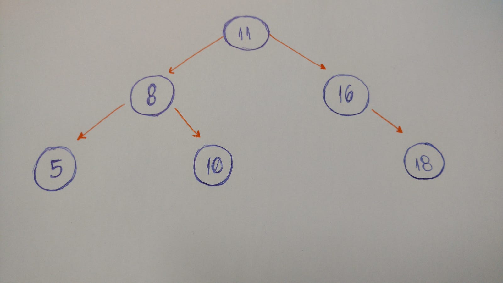
Now we will discuss a specific type of tree. We call it thebinary tree.

“In computer science, a binary tree is a tree data structure in which each node has at the most two children, which are referred to as the left child and the right child.” — Wikipedia

So let’s look at an example of a binary tree.

Let’s code a binary tree

The first thing we need to keep in mind when we implement a binary tree is that it is a collection of nodes. Each node has three attributes: value, left_child, and right_child.

How do we implement a simple binary tree that initializes with these three properties?

Let’s take a look.

class BinaryTree:
    def __init__(self, value):
        self.value = value
        self.left_child = None
        self.right_child = None

Here it is. Our binary tree class.

When we instantiate an object, we pass the value (the data of the node) as a parameter. Look at the left_child and the right_child. Both are set to None.

Why?

Because when we create our node, it doesn’t have any children. We just have the node data.

Let’s test it:

tree = BinaryTree('a')
print(tree.value) # a
print(tree.left_child) # None
print(tree.right_child) # None

That’s it.

We can pass the string ‘a’ as the value to our Binary Tree node. If we print the value, left_child, and right_child, we can see the values.

Let’s go to the insertion part. What do we need to do here?

We will implement a method to insert a new node to the right and to the left.

Here are the rules:

If the current node doesn’t have a left child, we just create a new nodeand set it to the current node’s left_child.
If it does have the left child, we create a new node and put it in the current left child’s place. Allocate this left child node to the new node’s left child.

Let’s draw it out. :)

Here’s the code:

def insert_left(self, value):
    if self.left_child == None:
        self.left_child = BinaryTree(value)
    else:
        new_node = BinaryTree(value)
        new_node.left_child = self.left_child
        self.left_child = new_node

Again, if the current node doesn’t have a left child, we just create a new node and set it to the current node’s left_child. Or else we create a new node and put it in the current left child’s place. Allocate this left child node to the new node’s left child.

And we do the same thing to insert a right child node.

def insert_right(self, value):
    if self.right_child == None:
        self.right_child = BinaryTree(value)
    else:
        new_node = BinaryTree(value)
        new_node.right_child = self.right_child
        self.right_child = new_node

Done. :)

But not entirely. We still need to test it.

Let’s build the followingtree:

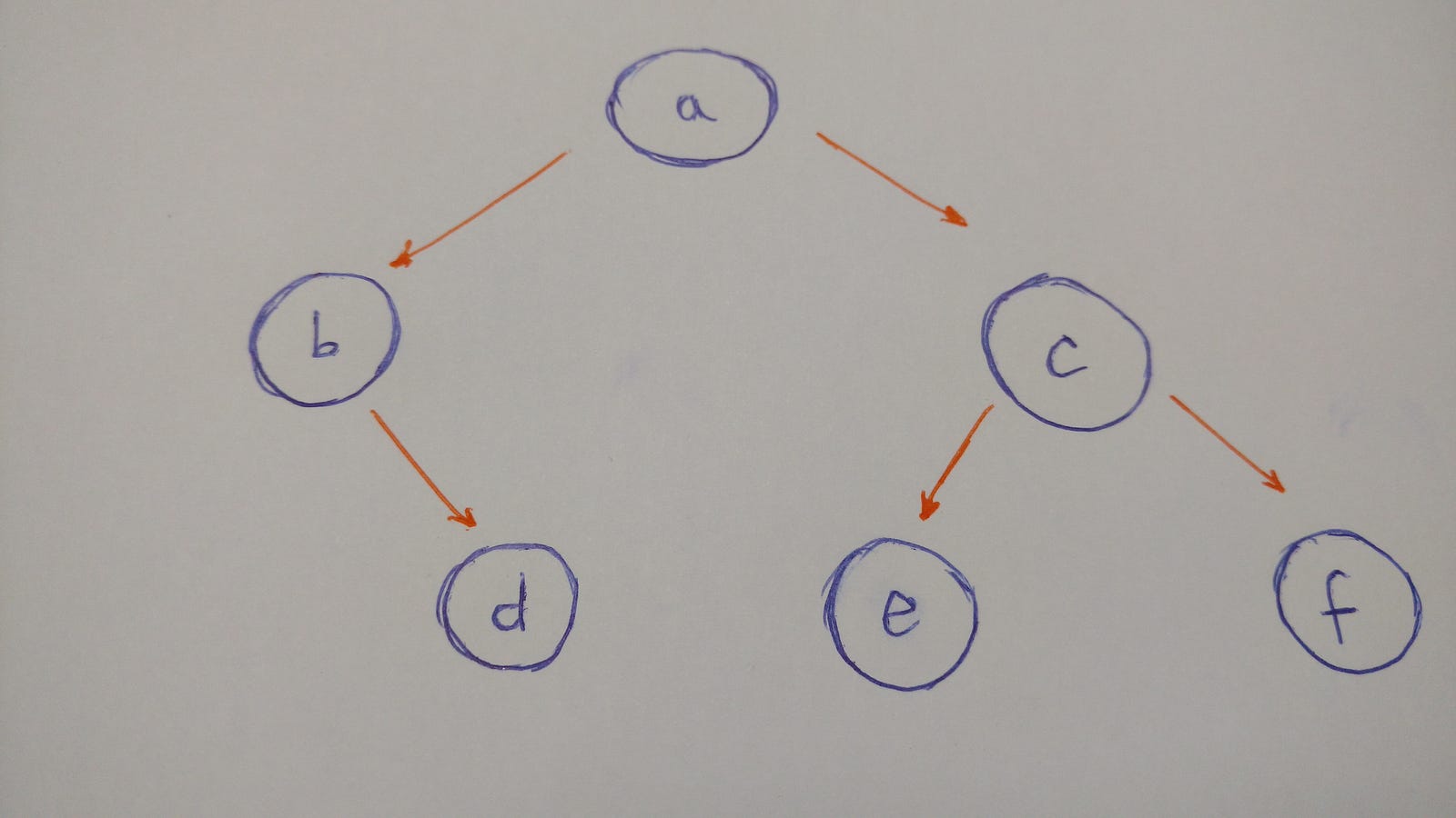
To summarize the illustration of this tree:

a node will be the root of our binary Tree
a left child is b node
a right child is c node
b right child is d node (b node doesn’t have a left child)
c left child is e node
c right child is f node
both e and f nodes do not have children

So here is the code for the tree:

a_node = BinaryTree('a')
a_node.insert_left('b')
a_node.insert_right('c')

b_node = a_node.left_child
b_node.insert_right('d')

c_node = a_node.right_child
c_node.insert_left('e')
c_node.insert_right('f')

d_node = b_node.right_child
e_node = c_node.left_child
f_node = c_node.right_child

print(a_node.value) # a
print(b_node.value) # b
print(c_node.value) # c
print(d_node.value) # d
print(e_node.value) # e
print(f_node.value) # f

Insertion is done.

Now we have to think about tree traversal.

We have two options here: Depth-First Search (DFS) and Breadth-First Search (BFS).

So let’s dive into each tree traversal type.

Depth-First Search (DFS)

DFS explores a path all the way to a leaf before backtracking and exploring another path. Let’s take a look at an example with this type of traversal.

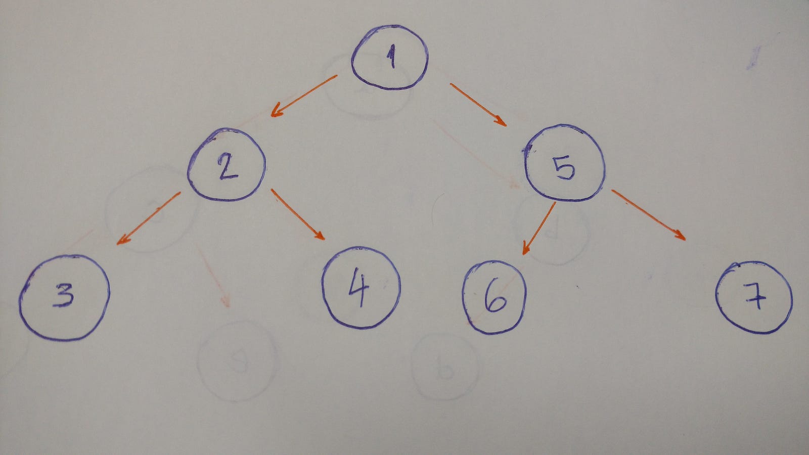
The result for this algorithm will be 1–2–3–4–5–6–7.

Why?

Let’s break it down.

Go to the left child (2). Print it.
Then go to the left child (3). Print it. (This node doesn’t have any children)
Backtrack and go the right child (4). Print it. (This node doesn’t have any children)
Backtrack to the root node and go to the right child (5). Print it.
Go to the left child (6). Print it. (This node doesn’t have any children)
Backtrack and go to the right child (7). Print it. (This node doesn’t have any children)
Done.

When we go deep to the leaf and backtrack, this is called DFS algorithm.

Now that we are familiar with this traversal algorithm, we will discuss types of DFS: pre-order, in-order, and post-order.

Pre-order

This is exactly what we did in the above example.

def pre_order(self):
    print(self.value)

    if self.left_child:
        self.left_child.pre_order()

    if self.right_child:
        self.right_child.pre_order()

In-order

The result of the in-order algorithm for this tree example is 3–2–4–1–6–5–7.

The left first, the middle second, and the right last.

Now let’s code it.

def in_order(self):
    if self.left_child:
        self.left_child.in_order()

    print(self.value)

    if self.right_child:
        self.right_child.in_order()

Post-order

The result of the post order algorithm for this tree example is 3–4–2–6–7–5–1.

The left first, the right second, and the middle last.

Let’s code this.

def post_order(self):
    if self.left_child:
        self.left_child.post_order()

    if self.right_child:
        self.right_child.post_order()

    print(self.value)

Breadth-First Search (BFS)

BFS algorithm traverses the tree level by level and depth by depth.

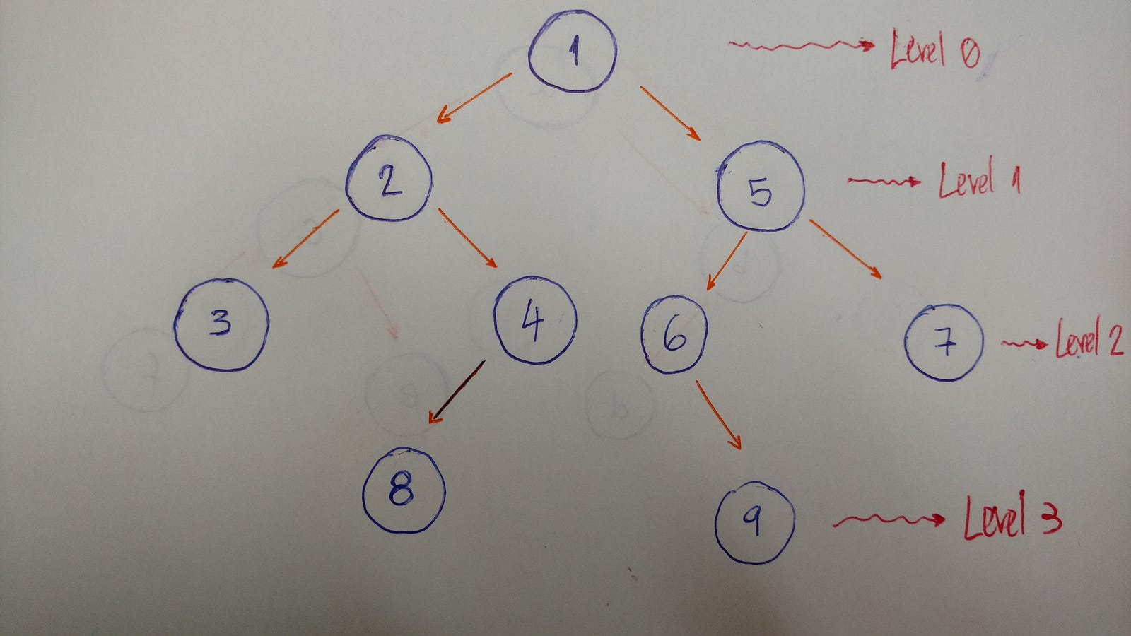
Here is an example that helps to better explain this algorithm:

So we traverse level by level. In this example, the result is 1–2–5–3–4–6–7.

Level/Depth 0: only node with value 1
Level/Depth 1: nodes with values 2 and 5
Level/Depth 2: nodes with values 3, 4, 6, and 7

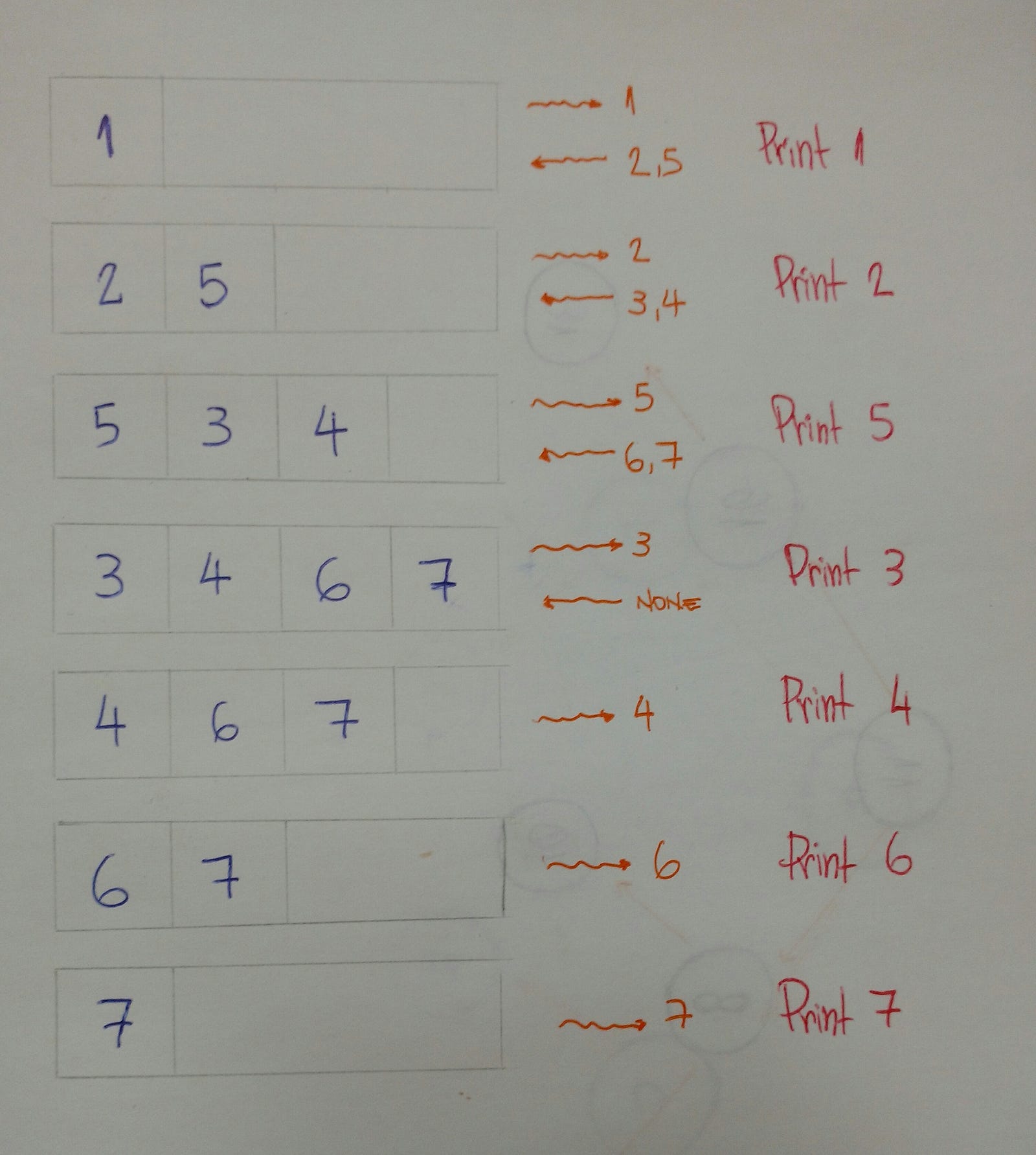
Now let’s code it.

def bfs(self):
    queue = Queue()
    queue.put(self)

    while not queue.empty():
        current_node = queue.get()
        print(current_node.value)

        if current_node.left_child:
            queue.put(current_node.left_child)

        if current_node.right_child:
            queue.put(current_node.right_child)

To implement a BFS algorithm, we use the queue data structure to help.

How does it work?

Here’s the explanation.

Binary Search tree

“A Binary Search Tree is sometimes called ordered or sorted binary trees, and it keeps its values in sorted order, so that lookup and other operations can use the principle of binary search” — Wikipedia

An important property of a Binary Search Tree is that the value of a Binary Search Tree nodeis larger than the value of the offspring of its left child, but smaller than the value of the offspring of its right child.”

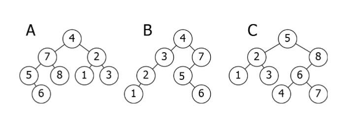
Here is a breakdown of the above illustration:

**A **is inverted. The subtree 7–5–8–6 needs to be on the right side, and the subtree 2–1–3 needs to be on the left.
**B **is the only correct option. It satisfies the Binary Search Tree property.
**C **has one problem: the node with the value 4. It needs to be on the left side of the root because it is smaller than 5.

Let’s code a Binary Search Tree!

Now it’s time to code!

What will we see here? We will insert new nodes, search for a value, delete nodes, and the balance of the tree.

Let’s start.

Insertion: adding new nodes to our tree

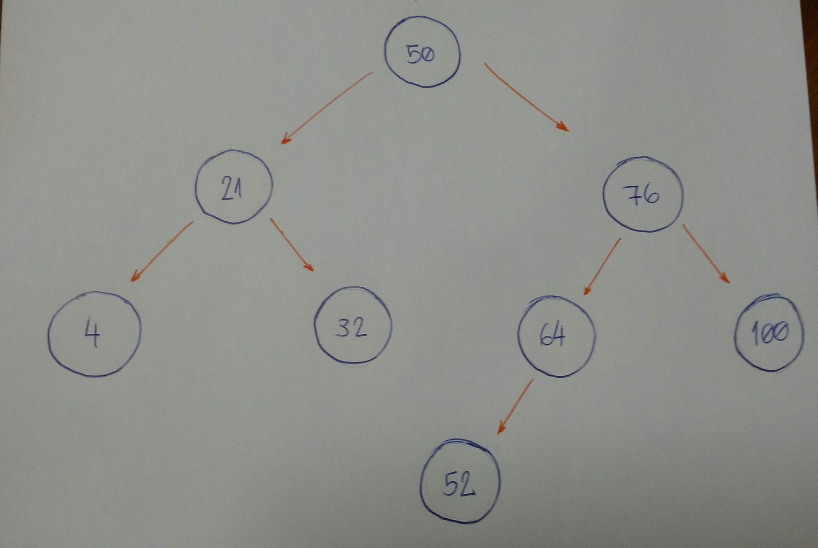
Imagine that we have an empty tree and we want to add new nodes with the following values in this order: 50, 76, 21, 4, 32, 100, 64, 52.

The first thing we need to know is if 50 is the root of our tree.

We can now start inserting node by node.

76 is greater than 50, so insert 76 on the right side.
21 is smaller than 50, so insert 21 on the left side.
4 is smaller than 50. Node with value 50 has a left child 21. Since 4 is smaller than 21, insert it on the left side of this node.
32 is smaller than 50. Node with value 50 has a left child 21. Since 32 is greater than 21, insert 32 on the right side of this node.
100 is greater than 50. Node with value 50 has a right child 76. Since 100 is greater than 76, insert 100 on the right side of this node.
64 is greater than 50. Node with value 50 has a right child76. Since 64 is smaller than 76, insert 64 on the left side of this node.
52 is greater than 50. Node with value 50 has a right child76. Since 52 is smaller than 76, node with value 76 has a left child 64. 52 is smaller than 64, so insert 54 on the left side of this node.

Do you notice a pattern here?

Let’s break it down.

Now let’s code it.

class BinarySearchTree:
    def __init__(self, value):
        self.value = value
        self.left_child = None
        self.right_child = None

    def insert_node(self, value):
        if value <= self.value and self.left_child:
            self.left_child.insert_node(value)
        elif value <= self.value:
            self.left_child = BinarySearchTree(value)
        elif value > self.value and self.right_child:
            self.right_child.insert_node(value)
        else:
            self.right_child = BinarySearchTree(value)

It seems very simple.

The powerful part of this algorithm is the recursion part, which is on line 9 and line 13. Both lines of code call the insert_node method, and use it for its left and right children, respectively. Lines 11 and 15 are the ones that do the insertion for each child.

Let’s search for the node value… Or not…

The algorithm that we will build now is about doing searches. For a given value (integer number), we will say if our Binary Search Tree does or does not have that value.

An important item to note is how we defined the tree insertion algorithm. First we have our root node. All the left subtree nodeswill have smaller values than the root node. And all the right subtree nodeswill have values greater than the root node.

Let’s take a look at an example.

Imagine that we have this tree.

Now we want to know if we have a node based on value 52.

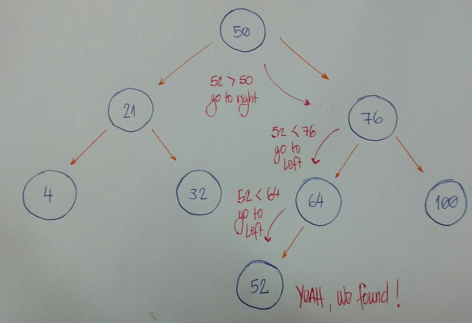
Let’s break it down.

Now let’s code it.

class BinarySearchTree:
    def __init__(self, value):
        self.value = value
        self.left_child = None
        self.right_child = None

    def find_node(self, value):
        if value < self.value and self.left_child:
            return self.left_child.find_node(value)
        if value > self.value and self.right_child:
            return self.right_child.find_node(value)

        return value == self.value

Let’s beak down the code:

Lines 8 and 9 fall under rule #1.
Lines 10 and 11 fall under rule #2.
Line 13 falls under rule #3.

How do we test it?

Let’s create our Binary Search Treeby initializing the root node with the value 15.

bst = BinarySearchTree(15)

And now we will insert many new nodes.

bst.insert_node(10)
bst.insert_node(8)
bst.insert_node(12)
bst.insert_node(20)
bst.insert_node(17)
bst.insert_node(25)
bst.insert_node(19)

For each inserted node , we will test if our find_node method really works.

print(bst.find_node(15)) # True
print(bst.find_node(10)) # True
print(bst.find_node(8)) # True
print(bst.find_node(12)) # True
print(bst.find_node(20)) # True
print(bst.find_node(17)) # True
print(bst.find_node(25)) # True
print(bst.find_node(19)) # True

Yeah, it works for these given values! Let’s test for a value that doesn’t exist in our Binary Search Tree.

print(bst.find_node(0)) # False

Oh yeah.

Our search is done.

Deletion: removing and organizing

Deletion is a more complex algorithm because we need to handle different cases. For a given value, we need to remove the node with this value. Imagine the following scenarios for this node : it has no children, has a single child, or has two children.

Scenario #1: A node with no children (leaf node).

#        |50|                              |50|
#      /      \                           /    \
#    |30|     |70|   (DELETE 20) --->   |30|   |70|
#   /    \                                \
# |20|   |40|                             |40|

If the node we want to delete has no children, we simply delete it. The algorithm doesn’t need to reorganize the tree.

Scenario #2: A node with just one child (left or right child).

#        |50|                              |50|
#      /      \                           /    \
#    |30|     |70|   (DELETE 30) --->   |20|   |70|
#   /
# |20|

In this case, our algorithm needs to make the parent of the node point to the child node. If the node is the left child, we make the parent of the left child point to the child. If the node is the right child of its parent, we make the parent of the right child point to the child.

Scenario #3: A node with two children.

#        |50|                              |50|
#      /      \                           /    \
#    |30|     |70|   (DELETE 30) --->   |40|   |70|
#   /    \                             /
# |20|   |40|                        |20|

When the node has 2 children, we need to find the node with the minimum value, starting from the node’sright child. We will put this node with minimum value in the place of the node we want to remove.

It’s time to code.

def remove_node(self, value, parent):
    if value < self.value and self.left_child:
        return self.left_child.remove_node(value, self)
    elif value < self.value:
        return False
    elif value > self.value and self.right_child:
        return self.right_child.remove_node(value, self)
    elif value > self.value:
        return False
    else:
        if self.left_child is None and self.right_child is None and self == parent.left_child:
            parent.left_child = None
            self.clear_node()
        elif self.left_child is None and self.right_child is None and self == parent.right_child:
            parent.right_child = None
            self.clear_node()
        elif self.left_child and self.right_child is None and self == parent.left_child:
            parent.left_child = self.left_child
            self.clear_node()
        elif self.left_child and self.right_child is None and self == parent.right_child:
            parent.right_child = self.left_child
            self.clear_node()
        elif self.right_child and self.left_child is None and self == parent.left_child:
            parent.left_child = self.right_child
            self.clear_node()
        elif self.right_child and self.left_child is None and self == parent.right_child:
            parent.right_child = self.right_child
            self.clear_node()
        else:
            self.value = self.right_child.find_minimum_value()
            self.right_child.remove_node(self.value, self)

        return True

To use the clear_node method: set the None value to all three attributes — (value, left_child, and right_child)

def clear_node(self):
    self.value = None
    self.left_child = None
    self.right_child = None

To use the find_minimum_value method: go way down to the left. If we can’t find anymore nodes, we found the smallest one.

def find_minimum_value(self):
    if self.left_child:
        return self.left_child.find_minimum_value()
    else:
        return self.value

Now let’s test it.

We will use this tree to test our remove_node algorithm.

#        |15|
#      /      \
#    |10|     |20|
#   /    \    /    \
# |8|   |12| |17| |25|
#              \
#              |19|

Let’s remove the node with the value 8. It’s a node with no child.

print(bst.remove_node(8, None)) # True
bst.pre_order_traversal()

#     |15|
#   /      \
# |10|     |20|
#    \    /    \
#   |12| |17| |25|
#          \
#          |19|

Now let’s remove the node with the value 17. It’s a node with just one child.

print(bst.remove_node(17, None)) # True
bst.pre_order_traversal()

#        |15|
#      /      \
#    |10|     |20|
#       \    /    \
#      |12| |19| |25|

Finally, we will remove a node with two children. This is the root of our tree.

print(bst.remove_node(15, None)) # True
bst.pre_order_traversal()

#        |19|
#      /      \
#    |10|     |20|
#        \        \
#        |12|     |25|

The tests are now done. :)

That’s all for now!

We learned a lot here.

Congrats on finishing this dense content. It’s really tough to understand a concept that we do not know. But you did it. :)

This is one more step forward in my journey to learning and mastering algorithms and data structures. You can see the documentation of my complete journey here on my Renaissance Developer publication.

Have fun, keep learning and coding.

Here are my Medium, Twitter & GitHub accounts.☺

Definition

Let’s dive into real life examples!

A technical definition

Terminology summary

Binary trees

Let’s code a binary tree

Depth-First Search (DFS)

Pre-order

In-order

Post-order

Breadth-First Search (BFS)

Binary Search tree

Let’s code a Binary Search Tree!

Insertion: adding new nodes to our tree

Let’s search for the node value… Or not…

Deletion: removing and organizing

That’s all for now!

Additional resources